The following has been updated from McVicar and Jupp (1998).
Remote sensing is the acquisition of digital data in the reflective, thermal or microwave portions of the electromagnetic spectrum (EMS). Measurements of the EMS are made either from satellite, aircraft or ground-based systems, but it is characteristically at a distance (or "remote") from the target. Due to the large spatial extent of the areas considered for the CRC for Sustainable Rice Production Project 1.1.05, this report will focus on data gathered from satellite remote sensing systems.
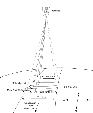
Remotely sensed images are recorded digitally by sensors on board the satellites. An example of a satellite operation is shown in Figure 1. The satellites vary in height above the Earth's surface from approximately 700 km, which orbit the earth, to some 36 000 km, which are geostationary above the equator. The images can be manipulated by computers to highlight features of soils, vegetation and clouds. Each pixel, or picture element, contributing to the image is a measurement of a particular wavelength of electromagnetic radiation at a particular spatial scale for a particular location at a specific time. The most common display of remotely sensed data is a single overpass, which non-remote sensing specialists may think of as a `satellite photo'.
|
Figure 1. Schematic of satellite operation, specifically the LANDSAT satellite and the Thematic Mapper (TM) sensor. [Adapted from (Harrison and Jupp, 1989). Reproduced by permission of CSIRO Australia].
When dealing with remotely sensed images, the extent, resolution, and density of the spectral, spatial and temporal characteristics need to be considered. Spectral extent describes what portion of the EMS is being sampled (e.g., is it just visible or does the range extend into the thermal). Spectral resolution refers to the bandwidths in which the sensor gathers information. Spectral density indicates the number of bands in a particular portion of the EMS (e.g., hyperspectral sensors have higher spectral density than broadband instruments). Spatial extent is the area covered by the image, while spatial resolution refers to the smallest pixel or picture element acquired. Spatial density refers to the amount of area measured by the sensor, so the spatial density for remotely sensed data is complete, while the spatial density of, for example, rainfall stations which are sampled at explicit points, would be incomplete. This means, for the extent of the image, remotely sensed data are a `census' at a particular spatial scale recorded at a specific time. Temporal extent is the recording period over which the data is available. For some systems, data has been recorded for over 25 years. Temporal resolution is the time that the data is acquired over. Remote sensors usually have a low temporal resolution (i.e., a matter of seconds), while rainfall data recorded at meteorological stations usually have a very high temporal resolution (i.e., they record almost continuously). Temporal density is the repeat characteristics of the satellite and, for some applications, greatly influences the availability of cloud free data.
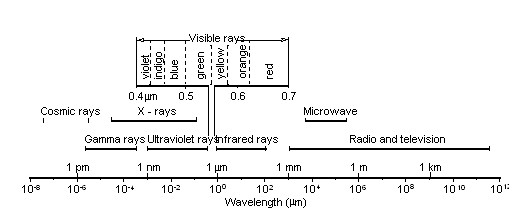
Remote sensing of the land surface occurs at wavelengths of the EMS where the light can pass through the Earth's atmosphere with no, or little interaction with the atmosphere. These bands of the EMS are called `atmospheric windows' and refer to the spectral extent in which radiation reaching remote sensing instruments carries information about the Earth's surface conditions. These `atmospheric windows' are defined by the transmittance of the constituents of the Earth's atmosphere. There are some gases, which absorb all electromagnetic radiation in certain wavelengths preventing these areas of the EMS being used for remote sensing. Figure 2 shows the divisions of the EMS briefly described in the next section.
|
Figure 2. Breakup of electromagnetic spectrum. Note that the scale is logarithmic. [Adapted from (Harrison and Jupp, 1989). Reproduced by permission of CSIRO Australia].
One basis of remote sensing is that different land covers have different spectral properties. Figure 3 shows idealised reflectance plots for two vegetation, soils and water types, respectively. Different surfaces also have varying responses in the thermal and microwave atmospheric windows of the EMS. Image processing approaches utilise these differences to extract information relevant for rice-based irrigation systems.
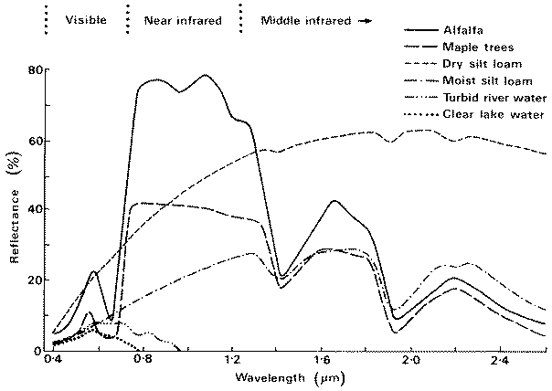
Figure 3. Idealised reflectance plots for different land cover types.
[Adapted from (Harrison and Jupp, 1989). Reproduced by permission of CSIRO Australia].
The reflective portion of the EMS ranges nominally from 0.4 to 3.75 micro meters (![]() m). Light of shorter wavelength than this is termed ultraviolet. The reflective portion of the EMS can be further subdivided into the visible 0.4 to 0.7
m). Light of shorter wavelength than this is termed ultraviolet. The reflective portion of the EMS can be further subdivided into the visible 0.4 to 0.7 ![]() m, near infrared (NIR) 0.7 to 1.1
m, near infrared (NIR) 0.7 to 1.1 ![]() m, and mid infrared 1.1 to 3.75
m, and mid infrared 1.1 to 3.75 ![]() m. It is in the visible portion of the EMS that we sense with our remote sensing device (eyes) which allow us to see. Different surface reflective properties allow us to distinguish colour in the visible region of the EMS.
m. It is in the visible portion of the EMS that we sense with our remote sensing device (eyes) which allow us to see. Different surface reflective properties allow us to distinguish colour in the visible region of the EMS.
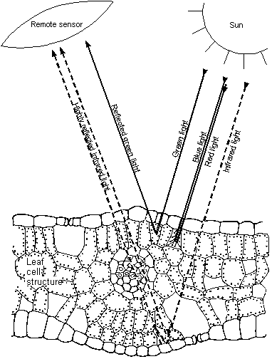
Chlorophyll pigments that are present in leaves absorb red light. In the NIR portion, radiation is scattered by the internal spongy mesophyll leaf structure, which leads to higher values in the NIR channels. This interaction between leaves and the light that strikes them, often determined by their different responses in the red and NIR portions of reflective light, see Figure 4, is how vegetation is detected using remote sensing. The objective of vegetation analysis from spectral measurements, often, is to reduce the spectral data to a single number that is related to physical characteristics of vegetation (e.g. leaf area, biomass, productivity, photosynthetic activity, or percent cover) (Baret and Guyot, 1991, Perry and Lautenschlager, 1984, Huete, 1988), while minimising the effect of internal (e.g. canopy geometry, and leaf and soil properties) and external factors (e.g. sun-target-sensor angles, and atmospheric conditions at the time of image acquisition) on the spectral data (Baret and Guyot, 1991, Chavez, 1988, Gong et al., 1992, Huete et al., 1985, Huete, 1987, Huete and Warrick, 1990, Huete and Escadafal, 1991, Kimes, 1983, Li et al., 1993, Richardson and Wiegland, 1977, Slater and Jackson, 1982, Singh, 1989).
|
Figure 4. Schematic reflectance of a typical green leaf in cross section; chloroplasts reflect the green light and absorb red and blue light for photosynthesis. Near infrared light is highly scattered by water in the spongy mesophyll cells.
[Adapted from (Harrison and Jupp, 1989). Reproduced by permission of CSIRO Australia].
Vegetation Indices (VI's) were developed in an attempt to obtain this objective from remote sensors by taking advantage of the differences in the reflective responses of vegetation in the red and NIR wavelengths. Although VI's are often hampered by limitations in dealing with the complex nature of real-life vegetation canopy interactions (Baret and Guyot, 1991, Huete et al., 1985, Huete, 1987, Huete and Jackson, 1987, Huete, 1988, Huete and Warrick, 1990, Huete and Escadafal, 1991, Huete et al., 1992, Qi et al., 1993), they have gained widespread popularity due to the benefits of remote sensing's high spatial density and extent, and the value added to generic, rather coarse-scale vegetation modelling.
LANDSAT Thematic Mapper (TM) and the Système pour l'observation de la Terre (SPOT) sensors, and many other remote sensing instruments, have channels situated in the red and NIR, see Table 1 and Figure 2. For example, the red and NIR bands for LANDSAT TM are band 3 (630-690 nm) and band 4 (769-900 nm), respectively. Most vegetation indices are combinations of these two reflective bands. The most common linear combinations are the simple ratio (NIR/Red) and Normalised Difference Vegetation Index (NDVI) = (NIR-Red)/(NIR+Red). Previous research has shown positive correlations exist between foliage presence, including measurements of LAI (Tucker, 1979, McVicar et al., 1996b, McVicar et al., 1996c, McVicar et al., 1996a) and plant condition (Sellers, 1985), and vegetation indices such as the simple ratio and NDVI. For a comprehensive listing of vegetation indices refer to Tian (1989), Kaufman and Tanre (1992), Thenkabail et al. (1994b) and Leprieur et al. (1996).
Table 1: General description of current and anticipated satellite sensors.
Some satellite specifications are available on the internet at sites like the Canadian Centre for Remote Sensing (CCRS) satellite details page
( http://www.ccrs.nrcan.gc.ca/ccrs/tekrd/satsens/sats/satliste.html).
Satellite: Sensor |
Channel # |
Spectral Resolution |
Spatial Resolution |
Sample Swath |
Repeat Cycle |
Lifetime |
Current |
||||||
NOAA:AVHRR1 |
1 |
580-680 nm |
1100 |
2700 km |
12 hrs |
1981 - present |
2 |
725-1100 nm |
" |
||||
3 |
3.55-3.93 |
" |
||||
4 |
10.3-11.3 |
" |
||||
5 |
11.5-12.5 |
" |
||||
SPOT:VMI2 |
1 |
430-470 nm |
1000 |
2000 km |
26 days |
1998- present |
2 |
500-590 nm |
" |
||||
3 |
610-680 nm |
" |
||||
4 |
790-890 nm |
" |
||||
5 |
1.58-1.75 |
" |
||||
LANDSAT:MSS3 |
4 |
500-600 nm |
80 |
185 km |
16 days |
1972- present |
5 |
600-700 nm |
" |
||||
6 |
700-800 nm |
" |
||||
7 |
800-1100 nm |
" |
||||
LANDSAT:(E)TM4 |
1 |
450-520 nm |
30 |
185 km |
16 days |
1983- present |
2 |
520-600 nm |
" |
(1999-present) | |||
3 |
630-690 nm |
" |
||||
4 |
769-900 nm |
" |
||||
5 |
1.55-1.75 |
" |
||||
7 |
2.08-2.35 |
" |
||||
6 |
10.4-12.5 |
120 (60) |
||||
(8) |
(520-900 nm) |
(15) |
||||
SPOT:HRV(IR)5 |
1 |
500-590 nm |
20 |
60 km |
26 days |
1986 - present |
2 |
610-680 nm |
" |
||||
3 |
790-890 nm |
" |
||||
4 |
510-730 nm |
10 |
||||
(4) |
(1.58-1.75 |
20 |
||||
(5) |
(610-680 nm) |
10 |
||||
IRS6 |
1 |
500-750 nm |
5.8 |
70 km |
22 days |
1997 - present |
2 |
520-590 nm |
23 |
140 km |
|||
3 |
620-680 nm |
" |
||||
4 |
770-860 nm |
" |
||||
5 |
1.55-1.70 _m |
70 |
||||
6 |
620-680 nm |
188 |
800 km |
|||
7 |
770-860 nm |
" |
||||
IKONOS7 |
1 |
450-520 nm |
4 |
13 km |
3 days |
1999-present |
2 |
520-600 nm |
" |
||||
3 |
630-690 nm |
" |
||||
4 |
760-900 nm |
" |
||||
5 |
450-900 nm |
1 |
||||
TERRA:ASTER8 |
1 |
520-600 nm |
15 |
60 km |
1-2 days |
1999-present |
2 |
630-690 nm |
" |
||||
3 |
760-860 nm |
" |
||||
4 |
1.60-1.70 _m |
30 |
||||
5 |
2.145-2.185 _m |
" |
||||
6 |
2.185-2.225 _m |
" |
||||
7 |
2.235-2.285 _m |
" |
||||
8 |
2.295-2.365 _m |
" |
||||
9 |
2.360-2.430 _m |
" |
||||
10 |
8.125-8.475 _m |
90 |
||||
11 |
8.475-8.825 _m |
" |
||||
12 |
8.925-9.275 _m |
" |
||||
13 |
10.25-10.95 _m |
" |
||||
14 |
10.95-11.65 _m |
" |
||||
TERRA:MODIS9 |
1 |
620-670 nm |
250 |
2330 km |
1-2 days |
1999-present |
2 |
841-876 nm |
" |
||||
3 |
459-479 nm |
500 |
||||
4 |
545-565 nm |
" |
||||
5 |
1.23-1.25 _m |
" |
||||
6 |
1.628-1.652 _m |
" |
||||
7 |
2.105-2.155 _m |
" |
||||
8 |
405-420 nm |
1000 |
||||
9 |
438-448 nm |
" |
||||
10 |
483-493 nm |
" |
||||
11 |
526-536 nm |
" |
||||
12 |
546-556 nm |
" |
||||
13 |
662-672 nm |
" |
||||
14 |
673-683 nm |
" |
||||
15 |
743-753 nm |
" |
||||
16 |
862-877 nm |
" |
||||
17 |
890-920 nm |
" |
||||
18 |
931-941 nm |
" |
||||
19 |
915-965 nm |
" |
||||
20 |
3.660-3.840 _m |
" |
||||
21 |
3.929-3.989 _m |
" |
||||
22 |
3.989-4.020 _m |
" |
||||
23 |
4.020-4.080 _m |
" |
||||
24 |
4.433-4.498 _m |
" |
||||
25 |
4.482-4.549 _m |
" |
||||
26 |
1.360-1.390 _m |
" |
||||
27 |
6.535-6.895 _m |
" |
||||
28 |
7.175-7.475 _m |
" |
||||
29 |
8.400-8.700 _m |
" |
||||
30 |
9.580-9.880 _m |
" |
||||
31 |
10.78-11.28 _m |
" |
||||
32 |
11.77-12.27 _m |
" |
||||
33 |
13.185-13.485_m |
" |
||||
34 |
13.485-13.785_m |
" |
||||
35 |
13.785-14.085_m |
" |
||||
36 |
14.085-14.385_m |
" |
||||
JERS:SAR10 |
1 |
1275 MHz |
18 x 18 |
75 km |
44 days |
1992-1996 |
JERS:OPS11 |
1 |
520-600 nm |
18 x 24 |
75 km |
||
2 |
630-690 nm |
" |
||||
3 |
760-860 nm |
" |
||||
4 |
760-860 nm |
" |
||||
5 |
1.60-1.71 _m |
" |
||||
6 |
2.01-2.12 _m |
" |
||||
7 |
2.13-2.25 _m |
" |
||||
8 |
2.27-2.40 _m |
" |
||||
ERS:SAR12 |
1 |
5.3 GHz |
<30 |
80-100 km |
Varies |
1991-present |
RADARSAT13 |
1 |
5.3 GHz |
28 x 25 |
100 km |
24 days |
1995-present |
Anticipated |
||||||
EROS:A14 |
1 |
500-900 nm |
1.8 |
12.5 km |
2 days |
2000 |
EROS:B15 |
1 |
500-900 nm |
0.82 |
16 km |
2 days |
2000 |
QUICKBIRD-116 |
1 |
450-900 nm |
1 |
704 km |
1-5 days |
2000 |
2 |
450-520 nm |
4 |
||||
3 |
520-600 nm |
" |
||||
4 |
630-690 nm |
" |
||||
5 |
760-890 nm |
" |
||||
ORBVIEW-3(4)17 |
* |
Panchromatic |
1 |
8 km |
3 days |
2000 |
* |
Multispectral |
4 |
||||
* |
Hyperspectral |
* |
5 km |
1 NOAA:AVHRR refers to a series of satellites operated by the United State Federal Agency, NOAA, National Oceanographic and Atmospheric Administration. The Advanced Very High Radiometric Resolution (AVHRR) sensor operates on this platform. From 1978 to 1981 only the first 4 channels were acquired. The NOAA series of satellites are polar orbiting at a height of some 700km, similar to the height of the LANDSAT series of satellites. AVHRR data is acquired over a large swath width, compared to the LANDSAT data, due to the wide scan angle, ![]() 55o, of the AVHRR sensor. The Local Area Coverage (LAC) pixel size is 1100 m at the sub-satellite point, becoming 5400 m at the of edge of the swath. Global Area Coverage (GAC) data are also recorded by the AVHRR sensor. GAC is a sub-sampling of the LAC data and nominally has a 5 by 3 kilometre resolution. GAC data is recorded onboard the satellite and recorded at the NASA Goddard Space Flight Centre. AVHRR/3 onboard NOAA-15 has a time shared Channel 3 referred to as 3a and 3b. Channel 3a has a spectral resolution from 1.58-1.64 _m and records during the day. Channel 3b has a spectral resolution from 3.55-3.93 _n and records at night.
55o, of the AVHRR sensor. The Local Area Coverage (LAC) pixel size is 1100 m at the sub-satellite point, becoming 5400 m at the of edge of the swath. Global Area Coverage (GAC) data are also recorded by the AVHRR sensor. GAC is a sub-sampling of the LAC data and nominally has a 5 by 3 kilometre resolution. GAC data is recorded onboard the satellite and recorded at the NASA Goddard Space Flight Centre. AVHRR/3 onboard NOAA-15 has a time shared Channel 3 referred to as 3a and 3b. Channel 3a has a spectral resolution from 1.58-1.64 _m and records during the day. Channel 3b has a spectral resolution from 3.55-3.93 _n and records at night.
2 SPOT:VMI refers to the Vegetation Monitoring Instrument (VMI) aboard the Système pour l'observation de la Terre 4 (SPOT4) satellite. The satellite has been functional from March 24, 1998 to present.
3 LANDSAT:MSS refers to the MultiSpectral Sensor (MSS) onboard the LANDSAT series of satellites. From 1972 to 1983, for LANDSAT 1 - 3 the repeat cycle was 18 days. LANDSAT is a polar orbiting sun synchronous satellite, which passes a given latitude at the same solar time, it operates at a height of 700 km.
4 LANDSAT:(E)TM refers to the Thematic Mapper (TM) sensor onboard LANDSAT 4 and 5 and the Enhanced Thematic Mapper (ETM) sensor onboard LANDSAT 7. Channel and wavelengths are not ascending due to the late inclusion of channel 7. In LANDSAT 7, the addition of a panchromatic band with a 15 meter spatial resolution is a notable change to previous LANDSAT sensors as is the increase in the thermal channel (6) spatial resolution to 60 meter. Daytime passes are at about 10:00 am local time, whereas night time passes are at about 10:45 pm.
5 SPOT:HRV(IR) refers to the Haute Resolution Visible (HRV) sensor aboard the Système pour l'observation de la Terre (SPOT) satellites 1-3 and the Haute Resolution Visible Infrarouge (HRVIR) aboard the SPOT 4 satellite. SPOT 1 lifetime is from February 22, 1986 to present. SPOT 2 has been transferring data from January 21, 1990 until present, and SPOT 3 was functional from September 26, 1993 to November 14, 1996 when the satellite was declared lost. There has been an addition of a new Channel between 1.58-1.75 μm with a 20 m spatial resolution and a change of the 10 m panchromatic Channel from 510-730 nm in SPOT 1-3 to 610-680 nm in SPOT 4. The satellite has been functional from March 24, 1998 to present. Text inside parenthesis represent the changes in SPOT 4.
6 IRS refers to the Indian Remote Sensing (IRS) satellite 1-D. The IRS-1D was launched into polar orbit on the 29th of September, 1997. It's payload has been activated since October, 1997. This satellite contains a panchromatic sensor, a LISS-III sensor detecting VIS, NIR, and SWIR, and a WiFS sensor collecting red and NIR.
7 IKONOS refers to Space Imaging's IKONOS satellite launched September 24, 1999
8 TERRA:ASTER refers to the Advanced Spaceborne Thermal Emission and Reflection (ASTER) radiometer instrument aboard the TERRA (EOS AM-1) satellite. ASTER is designed to obtain detailed maps of land surface temperature, emissivity, reflectance and elevation. ASTER is the only high spatial resolution instrument on the TERRA platform.
9 TERRA:MODIS refers to the Moderate Resolution Imaging Spectroradiometer (MODIS) instrument aboard the TERRA (EOS AM-1) satellite. MODIS will view the Earth's surface every 1-2 days in 36 spectral bands. Spatial resolution varies from 250m to 1000m. MODIS is geared to global change models.
10 JERS:SAR refers to the Synthetic Aperature Radar (SAR) sensor on-board the Japan Earth Resources Satellite 1 (JERS-1) satellite. Satellite life was from February 11, 1992 to October 12, 1998. The first SAR image was recived on April 21, 1992. A cooling device failed in January of 1994 disrupting steady state transmission.
11 JERS:OPS refers to the Optical Sensors (OPS) on-board the Japan Earth Resources Satellite 1 (JERS-1) satellite. Channel 4 is for forward viewing (15.53_). Channel 3 and 4 make a stereo pair. Satellite life was from February 11, 1992 to October 12, 1998. The first SAR image was recived on April 21, 1992. A cooling device failed in January of 1994 disrupting steady state transmission.
12 ERS:SAR refers to the Active Microwave Instrumentation (AMI) sensor aboard the European Remote Sensing (ERS) 1 and 2 satellites. The information given in the table is for Synthetic Aperture Radar (SAR) in image mode (5.3 GHz C-Band). Repeat cycle has been variable: 3 day cycle from July 17, 1991 to March 1, 1992, 35 day cycle from March 2, 1992 to December 22, 1993, 3 day cycle from December 23, 1993 to April 9, 1994, 168 day cycle from April 10, 1994 to March 20, 1995, 35 day cycle from March 21, 1995 to present.
13 RADARSAT refers to the Canadian Space Agency's RADARSAT satellite in standard mode. RADARSAT collects Synthetic Aperature Radar (SAR) in the C-Band at an incidence angle of 20-49_, nominal spatial resolution of 30m, and swath of 100 km. There are 5 other operating modes including wide swath (20-45_, 30m, 150 km), fine resolution (37-47_, 8m, 45 km), extended coverage (52-58_, 18-27m, 75 km), scanSAR narrow (20-49_, 50m, 300 km), and scanSAR wide (20-49_, 100m, 500 km)
14 EOS:A refers to the 1.8 meter panchromatic satellite due to be launched in 2000 by West Indian Space.
15 EOS:B refers to the 0.82 meter panchromatic satellite due to be launched in 2000 by West Indian Space.
16 QUICKBIRD-1 refers to EarthWatch Inc.'s satellite due to be launched sometime in this year (2000). QuickBird is designed to have 1 meter panchromatic and 4 meter multispectral spatial resolution.
17 ORBVIEW-3(4) refers to Orbital Imaging's Orbview-3 and Orbview-4. Also meant to launch sometime in 2000, both will gather 1 meter panchromatic and 4 meter multispectral. Orbview-4 will also collect hyper spectral data in 200 wavebands. Some specific spectral and spatial information is unknown at this time (*).
While the amount of leaf is one determinant of the signal strength in the reflective portion of the EMS there are several other important factors which control the acquired value. These include the sun-target-sensor geometry. This will control the amount of shadow contributing to the signal; the shadow may be driven by insolation effects due to regional topography and may also be influenced by vegetation shadowing. This effect, termed the bidirectional reflectance distribution function (BRDF) (Burgess and Pairman, 1997, Deering, 1989), is characteristic of vegetation structure. Other effects in the reflective portion of the EMS include changes in soil colour and changes in the observed signal due to changes in the atmospheric component of the signal, including atmospheric precipitable water (Choudhury and DiGirolamo, 1995, Hobbs, 1997), atmospheric aerosols (e.g., dust), and changes in the response of the sensor over time.
Primarily, the reflective portion of the EMS has been used for:
1. identification of rice;
2. area estimation of rice;
3. estimation and prediction of crop yield; and
4. crop damage assessment
These are discussed more fully in section 3.1, 3.2, 3.3 and 3.4, respectively.
The microwave portion of the EMS ranges nominally from 0.75 to 100 centimetres. Radio signals have wavelengths that are included in these bands. These systems can either be active (the sensor sends its own signal) or passive (the background signal from the Earth's surface is observed). There are five smaller sections of this range which are used for remote sensing. These are :
P band 100 - 30 cm;
L band 30 - 15 cm;
S band 15 - 7.5 cm;
C band 7.5 - 3.75 cm; and
X band 3.75 - 2.4 cm.
RADAR (RAdio Detection And Ranging), is an active system based upon sending a pulse of microwave energy and then recording the strength, and sometimes polarisation, of the return pulses. The way the signal is returned provides information to determine characteristics of the landscape. RADAR has been used in the determination of near surface soil moisture, and the identification of rice crops based on the presence of standing water.
Primarily, the microwave portion of the EMS has been used in agriculture for:
1. identification of rice
2. area estimation of rice; and
3. estimation and prediction of crop yield.
These are discussed more fully in sections 3.1, 3.2, and 3.3, respectively.
The thermal portion of the EMS ranges nominally from 3.75 to 12.5 micro meters. The radiant energy observed by sensors is emitted by the surface, be it land, ocean or cloud top, and is a function of surface temperature. Models have been developed to allow surface temperature to be extracted from thermal remote sensing. Prata et al. (1995) review the algorithms and issues involved in the calculation of land surface temperatures, denoted Ts.
Thermal remote sensing is an instantaneous observation of the status of the surface energy balance (SEB). The SEB is driven by the net radiation at the surface. During the daytime this is usually dominated by incoming shortwave radiation from the sun, the amount reflected depending on the albedo of the surface. There are also up and down welling longwave components. At the ground surface, the net allwave radiation is balanced between the sensible, latent and ground heat fluxes. Over long periods of time the ground heat flux averages out, and the SEB represents the balance with the sensible and latent heat fluxes. During the day the measured surface temperature at the Earth's surface is, in part, dependent on the relative magnitude of the sensible and latent heat fluxes.
The surface energy balance at any instant is given by:
|
(1) |
where:
Rn is net all wavelength radiation (Wm-2);
_E is the latent heat flux (of evapotranspiration (ET)) (W m-2);
H is the sensible heat flux (W m-2), or the energy involved in the movement of the air and its transfer to other objects (such as trees, grass etc); and
G is the ground heat flux into the soil or other storages (W m-2).
_E denotes the amount of energy needed to change a certain volume of water from liquid to vapor, either by transpiration or evaporation. The combination of these two fluxes is called evapotranspiration. The net available energy (AE) at the Earth's surface, which is available for conversion to other forms, can be written as:
|
(2) |
where the terms are defined as above. A key factor determining the observed surface temperature is the partitioning of the AE into the latent and sensible heat fluxes. This is governed by the amount of water available and the ease with which it is transferred from the surface to the atmosphere, via _E. See Eymard and Taconet (1995), and the reference list therein, for a review of methods to infer surface fluxes from satellite data. These techniques provide the opportunity to map the actual _E flux, denoted _Ea. For given meteorological conditions there will also be a potential _E, denoted _Ep, which could occur if water was not limiting. The ratio of _Ea to _Ep is termed the moisture availability (ma).
Thermal remotely sensed data can also be recorded at night. During the night the SEB is dominated by the release of heat from the ground, which was absorbed during the daylight hours. The release of heat during the night is governed by how much was absorbed during the day and, the rate at which it is released after sunset. This is a function of the environment's capacity to store heat, which also depends on the amount of water stored in the environment.
The thermal portion of the EMS has been used to determine:
1. surface temperature estimation (including water temperature); and
2. moisture availability (ma) mapping.
These are discussed more fully in sections 3.4 and 3.5.
Remotely sensed data (visible, thermal, microwave), GIS data layers (soils, geology), point based measurements (rainfall, soil moisture, biomass) or model outputs (biomass, soil moisture) all have spatial and temporal attributes associated with the data attribute, and can be integrated. Economic situations and social indicators will have a time and may have a space associated with the data attribute and can also be integrated. The integration of several data types will allow factors such as crop types, yield estimates, and water use to be determined more objectively.
Many GIS data layers cover entire regions. However, these are often produced from the spatial interpolation of point samples; this is especially the case for some meteorological surfaces. Some physical parameters, such as soil water holding capacity, which are assumed to be time in-variant, only need to be mapped once. Remote sensing provides repeated measurements, at a particular spatial scale and electromagnetic wavelength, which allows dynamic environmental conditions, such as soil moisture and vegetation cover, to be monitored.
The data structure in the GIS can be conceptualised as being pancakes of remotely sensed data (TM or SPOT), which are intersected at right angles by skewers of point based data (Bureau of Meteorology (BOM) rainfall and air temperatures). In the data, two dimensions (the pancakes) are spatial, latitude and longitude, and the third (the skewer) is time. For some issues (e.g., groundwater monitoring) it can be important to include elevation (or depth) as another dimension in the data structure. Both data sets (point based BOM and remotely sensed) often have vastly different spatial and temporal scales. For example, TM data are spatially dense, with a 30 metre spatial resolution, and are recorded over large areas in a matter of seconds at a specific time for specific wavelengths. This means, for the extent of the image, remotely sensed data are a `census' (high spatial density) at a particular spatial scale recorded at a specific time. Depending on the amount of cloud coverage and the satellite repeat characteristics, optical remotely sensed data may only be available monthly (low temporal density). On the other hand, meteorological data are recorded at specific points, which may be separated by tens to hundreds of kilometres (low spatial density). Meteorological variables are usually recorded daily (high temporal density), as either integrals (e.g., rainfall and wind-run totals), or extremes (e.g., maximum and minimum air temperatures). Thus, remotely sensed data are spatially dense but temporally sparse, while meteorological data are spatially sparse but temporally dense.
Data of varying degrees of spatial and temporal density can be incorporated into a GIS. Spatial and temporal resolutions of the data will vary, depending on, among other things, the issues being addressed. See Langran (1992), Peuquet (1994), Peuquet (1995) and Mitasova et al. (1995), for detailed discussions of both the theoretical and the technical aspects of data integration arising from the inclusion of time in GIS.
The advantages of using time series of several data sets, including those not observed remotely, is illustrated in the following example from Barrs and Prathapar (1994) and Barrs and Prathapar (1996). An irrigation company may want to estimate crop area in order to plan for the marketing of specific crops. To get an early estimate of rice production, a November image was acquired, in which standing water was used to estimate rice area. Standing water can be easily identified in the NIR portion of the EMS where it has a low reflectance (see Figure 3). In order to map other crop types and to delineate standing water areas on which rice was not grown, a March image well into the rice growing season was then acquired. This image was used to refine the end of season yield prediction by `fine-tuning' the irrigated area estimation from the first image. By determining areas that were still standing water, they could ascertain that these were either failed crops or permanent water bodies. The later image was also used to classify other summer crop types, with varying confidence. Other GIS data, like field delineations and known water bodies, could also have been used to adjust the classification. Errors of omission as well as errors of commission can be corrected, increasing classification accuracy. For example, in a land use map, if 90% of a known field is classified as rice, it makes sense to assume the whole field is rice, thus fixing some errors of omission. However, in a land cover map, knowing, for example, that 10% of the paddock planted with rice did not grow successfully can be valuable information for estimating yields, thus fixing some possible errors of commission. The difference between land use and land cover should be noted as these should not be combined in thematic classes.
It should be noted that some data likely to be used in spatial modelling will not have a precise spatial reference associated with it, for example economic factors such as interest rates and grain prices. However, the temporal nature of these variables can be incorporated into larger information systems, of which remotely sensed data are but one component.